HW 8 -- POMDPs and Bandits

The questions below are due on Wednesday April 22, 2026; 11:59:00 PM.
 

There is no programming component for this homework.

This homework focuses on partially observable decision making and bandits: the belief simplex and optimal policies for a robot charger POMDP, sparse sampling, multi-armed bandits, and two longer modeling problems.

1) Belief Simplex§

In this section we will discuss a useful representation for visualizing a set of beliefs, called the "Belief Simplex".

Specifically, the set of possible belief states over K world states is a simplex, which is a K-1 dimensional manifold (surface) embedded in the K dimensional space. In our case where K = 3, we can visualize a belief space in a 3D plot. In the following simplex visualizations, you will see green areas covering part of the belief space, which indicates the set.

The figure above shows an illustration of what a simplex looks like in 3D. Figure credit: blog.bogatron.net.

1. For each of the following belief states, explain what part of the simplex it corresponds to.

   • b(s = 0) = 1 -- A vertex An edge A line that is not an edge A triangle

     

   • b(s = 0) = 0 -- A vertex An edge A line that is not an edge A triangle

     

   • b(s = 0) > p -- A vertex An edge A line that is not an edge A triangle

     

   • b(s = 0) = b(s = 1) -- A vertex An edge A line that is not an edge A triangle

     

Recall the robot-charger POMDP: Our robot has lost its charger! The robot lives in a world with K=3 locations but it needs to have the charger in location 0 (where the power outlet is) in order to plug it in and charge.

The robot doesn't have any uncertainty about its own location (and we won't model that) but it does have uncertainty about the location of the charger. When the robot looks in location loc, by executing a look(loc) action, it will receive an observation in \{0, 1\}. The low battery means that its sensors aren't working very well.

• If the charger is in the location loc, it will get observation 1 with probability 0.9.
• If the charger is not in location loc, it will get observation 1 with probability 0.4.

The robot can also try to execute a move(loc1, loc2) (which moves the charger):

• If the charger is actually in loc1, then with probability 0.8, the charger will be moved to loc2, otherwise, it will stay in loc1.
• If the charger is not in loc1, then nothing will happen.

Because of the constraints of the robot's arm, we can't do all possible move actions. Specifically, the only valid movements are move(0, 1), move(1, 2), and move(2, 0).

The robot has two more actions (charge and nop)

• If it executes the charge action when the charger is in location 0, then it gets a reward of 10 and the game terminates.
• If it executes that action in any other state, it gets reward -100 and the game terminates.

It gets reward -0.1 for every look action and -0.5 for every move action in all other states.

Finally, it has a nop action, with reward 0, which does not provide a useful observation, and does not affect the world state.

For actions that don't yield useful information about the environment (move, charge, and nop), we assume that they get observation 0 with probability 1, independent of the state.

2. Which of the following plots corresponds to belief states in which the value of charging is greater than 0?

   A	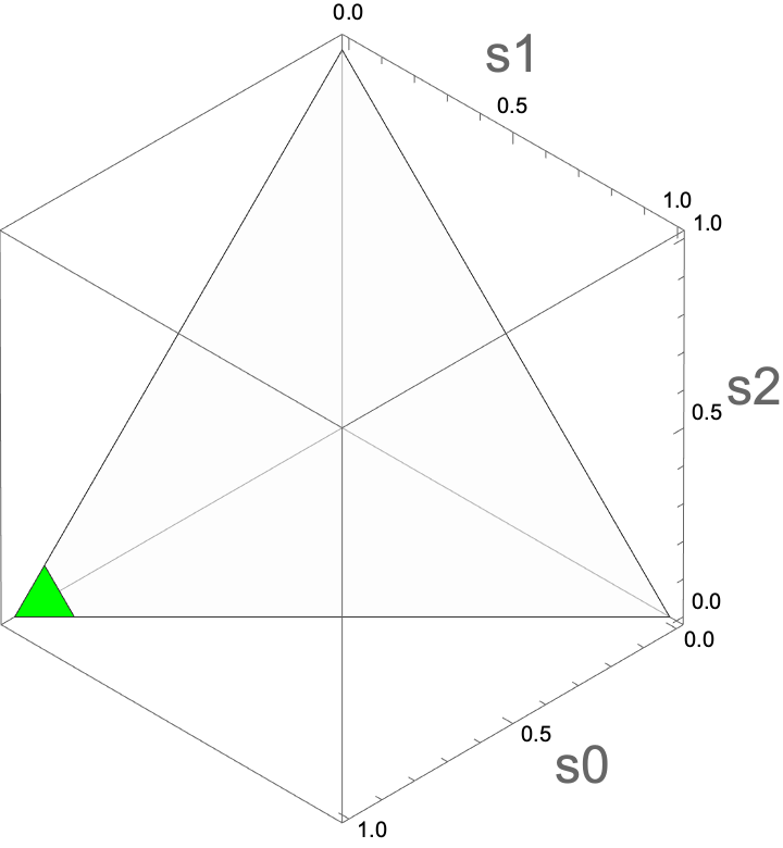	B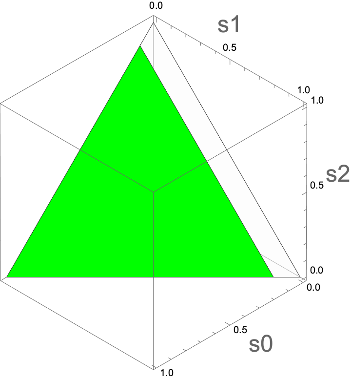
   C	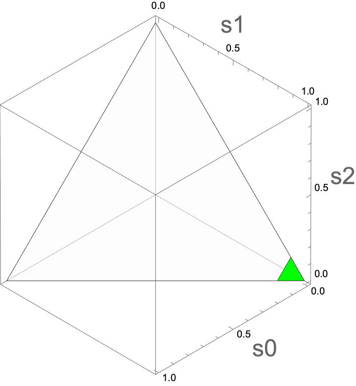	D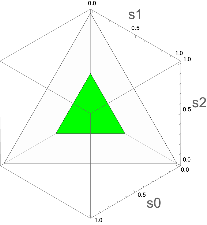

   Select the simplex in which the value of charging is greater than 0.

   Pick one. -- A B C D

   

2) Optimal Solution§

2.1) Counting§

In general, consider a Partially-Observable Markov Decision Process (POMDP) with action space \mathcal{A} and observation space \mathcal{Z} with horizon h. One way to compute the "optimal" strategy for solving the POMDP is to build a "policy tree". Denote A = |\mathcal{A}| and Z = |\mathcal{O}|.

1. What's the size of the policy tree of horizon h?

   	O(A^h)
   	O(Z^h)
   	O((AZ)^h)
   	O(A^{(Z^h)})

   

2. How many possible policy trees of horizon h are there?

   	O(A^h)
   	O(Z^h)
   	O((AZ)^h)
   	O(A^{(Z^h)})

   

3. Are there any algorithms for solving POMDPs optimally with a better worst-case complexity than a SPA (Stupidest Possible Algorithm)?

   	Yes! :-)
   	No... :-(

   

2.2) Belief Simplex Visualization of Optimal Policies§

Here are four plots showing the optimal finite-horizon policies with \gamma = 1.0 for horizons H = 1, 2, 3, 4. The colors correspond to actions:

• Green: look(0)
• Magenta: look(1)
• Cyan: look(2)
• Red: move(0, 1)
• Blue: move(1, 2)
• Orange: move(2, 0)
• Brown: charge
• Grey: nop

H=1		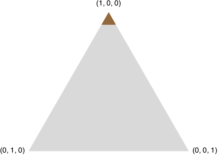H=2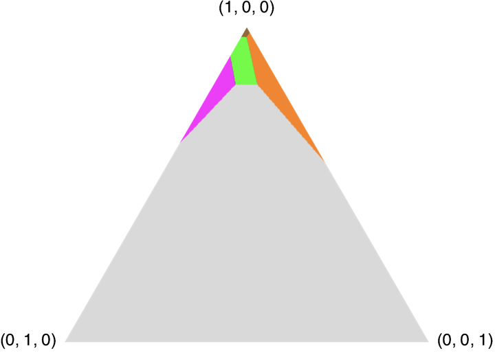
H=3		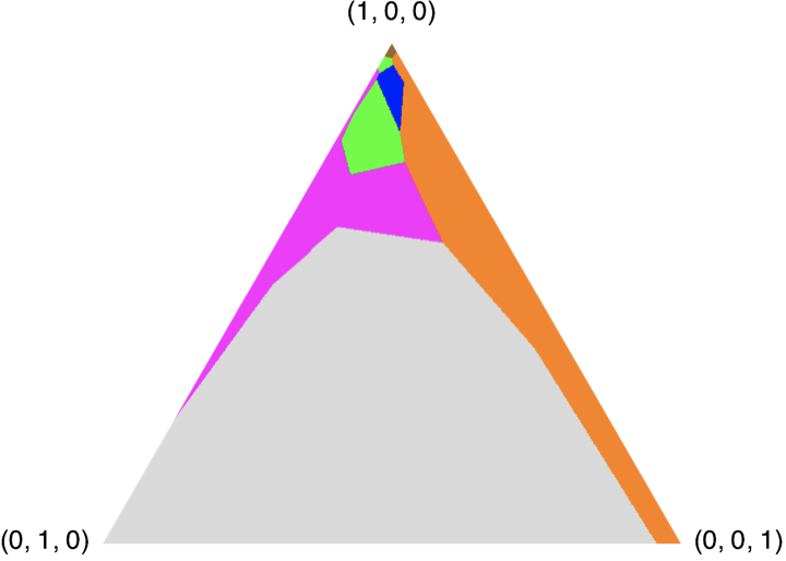H=4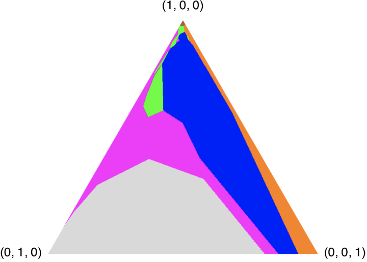

Note: Red and cyan have never appeared in the figures above, but they may appear in figures showing the optimal policies for longer horizons.

2. The horizon 2 policy has 5 regions. In which regions are we guaranteed to charge on this step or the next one? (Hint: look at the simplex, and use your intuition about the workings of the charge POMDP.)

   Mark all colors that apply.

   	Brown
   	Green
   	Magenta
   	Orange
   	Grey

   

3. The horizon 2 policy has 5 regions. In which regions will we charge on the next step if we get observation 1 on this step?

   Mark all colors that apply.

   	Brown
   	Green
   	Magenta
   	Orange
   	Grey

   

4. In the horizon 2 policy, there are fewer belief states when we want to charge than there are in the horizon 1. Why?

   Mark all reasons that apply.

   	Because discounting makes charging less attractive now
   	Because we have time to increase our belief that the charger is in location 0
   	Because we lose information over time

   

5. Is it true that, in the horizon 2 policy, for all the gray belief states, there is no possible observation that would put us in the brown region of the horizon 1 policy?

   Enter True or False.

   	True
   	False

   

6. If we were to decrease the cost for looking, would the magenta region in the horizon 2 policy be bigger, smaller, or the same?

   Mark the change to the magenta region.

   	Bigger
   	Smaller
   	Same

   

3) Sparse Sampling Theory§

Proving an error bound on the sparse sampling algorithm is beyond our scope, but let’s consider a simpler case, with horizon 1. So, really, we are interested in a contextual bandit problem.

• We find ourselves in a state s.
• There are only two actions.

Normally, we would compute Q(s, a) = \sum_{s'} R(s, a, s') P(s' | s, a) for each action and select the action with the largest expected reward. But what if the number of possible next states is so large that we can’t afford to compute Q? We can draw n samples s'_i \sim P( \cdot | s, a), where i=1,2,\cdots,n and estimate

\hat{Q}(s, a) = \frac{1}{n} \sum_{i=1}^n R(s, a, s'_i).

Assume that 0 < R(s, a, s’) < \mathrm{Rmax} for all s, a, s’. Let's think about how far wrong our estimate \hat{Q} can be from the true Q value.

Note that we're developing the general case, but for your answers in this question, you can assume that \mathrm{Rmax} = 1.

Chernoff and Hoeffding to the rescue! The idea of tail bounds from probability, which tell us (assuming independent samples) how the quality of our estimates depends on the size of the sample set. One version of their bound, applied to our problem, says that if we estimate \hat{Q} as above, then

P(|\hat{Q}(s, a) - Q(s, a)| \ge \epsilon) \le 2 \exp(-2n\epsilon^2 / \mathrm{Rmax}^2).

1. What's the upper bound for Q(s, a) for all s and a?

   Please input your answer as a number.
   

   

2. You want to be at least 95% sure that your \hat{Q} estimates differ from the correct value by at most 0.1, how many samples would you need to take (at least)?

   Please input your answer as a single integer.
   

   

3. How does the required number of samples, n, change if the size of state space S increases?

   	Increase
   	Decrease
   	Not Change

   

4. What will happen to n if you want your estimates to differ from the correct value by at most 0.01 with probability 95%?

   	Increase by a factor of 10
   	Increase by a factor of 100
   	Increase by a factor of 1000
   	Decrease by a factor of 10
   	Decrease by a factor of 100
   	Decrease by a factor of 1000
   	Not Change

   

5. How does n roughly change by (relative to part 4) if you want to be 99% sure your estimates differ from the correct value by at most 0.01?

   	Increase by a factor of 2
   	Increase by a factor of 10
   	Decrease by a factor of 2
   	Decrease by a factor of 10
   	Not Change

   

4) Bandit§

1. Recall the super-simple bandit problem from lecture. There are K arms with binary reward. For each arm i, the probability of payoff is randomly picked to be one of \{0.1, 0.5, 0.9\}. In the super-simple bandit example, which of the following priors would mean that we couldn't maintain a factored belief representation?

   	For each arm, P(p_i = .1) = .8, P(p_i = .5) = .1, P(p_i = .9) = .1
   	We know that all the arms are identical to each other, so with probability 1/3 all p_i=.1, with probability 1/3 all p_i=.5, and with probability 1/3 all p_i=.9
   	One arm has the prior P(p_i = .1) = .5, P(p_i = .5) = .5. For other arms, P(p_i = .1) = .8, P(p_i = .5) = .1, P(p_i = .9) = .1

   

2. What would happen if we tried using the most-likely observation determinization on a Bernoulli bandit problem?

   Mark all that are true.

   	It actually wouldn't apply because the underlying POMDP state space is infinite.
   	Assuming there are only two arms, it would always make one of two plans: always pick right arm or always pick left arm.
   	It would behave the same way as always picking the arm with the most total successes.
   	It would behave the same way as always picking the arm with the highest ratio of \alpha / (\alpha + \beta) where \alpha, \beta are the parameters of the posterior beta distribution.

   

3. What is the best known upper bound on the regret, as a function of trial length N, of the following K-arm bandit strategies?

   Thompson sampling

   	O(1)
   	O(\log N)
   	O(\sqrt{N})
   	O(N)

   
   UCB strategy that picks the arm with maximum \hat{\mu_i} + \sqrt{\frac{2 \log(1 + N \log^2 N)}{N_i}}

   	O(1)
   	O(\log N)
   	O(\sqrt{N})
   	O(N)

   

4. Consider the two-arm bandit problem where the mean reward for each arm is drawn uniformly from [0, 1]. Compute the exact regret of the following strategies over n actions.

   Picking an arm at random and sticking with it the whole time. Compute the exact regret, not the asymptotic. Write your expression in terms of n.
   

   
   Picking an arm at random on each step. Compute the exact regret, not the asymptotic, for the two-arm bandit case. Write your expression in terms of n.
   

   

5. Consider all possible bandit strategies that involve interacting with the arms for a constant number of steps K (independent of N) and using that information to pick a single arm to execute for the rest of the trial.

   Are some of these strategies asymptotically better than picking an arm uniformly at random?

   	Yes
   	No

   

5) Robot Grid World§

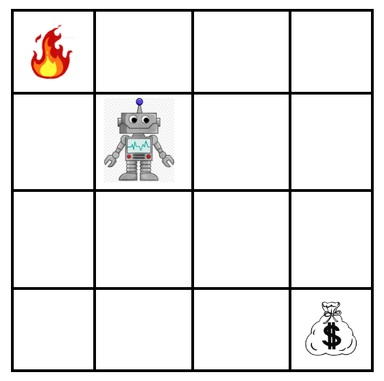
Consider the following gridworld containing a robot, a large positive reward (the money, worth +1000 points) and a large negative reward (the flames, worth -1000 points). The robot is trying to obtain the money and avoid the flames.

The robot's orientation is fixed, but it can move up, down, left and right, and each action costs -1 points. However, it cannot directly observe its (x, y) position --- it can only observe whether there are any walls next to it in the four compass directions. For instance, if the robot were in the top right corner, it would see a wall to the north and to the east. It would also know unambiguously that it is in that cell --- no other cells have a wall to the north and to the east.

There are only walls around the boundary of the gridworld --- there are no internal walls. The problem ends when the robot obtains the money or is consumed by flames.

Assume that the robot initially has no knowledge of its position. Assume the robot's motion dynamics are perfect --- when it attempts to move in a given direction, the motion occurs deterministically, unless there is a wall in the way. Assume sensing is perfect.

The robot's (unobservable) start location is at state (1, 2), using the convention that the bottom-left corner is (0, 0). The money is in the bottom-right reachable cell and the flames in the top-left, as in the figure below.

5.1) Belief and planning§

1. How many distinct belief states are reachable from the initial uniform belief, including the start belief? (If you wish, you may count or exclude beliefs where the episode has already ended; use the count that includes those terminal beliefs.)

   Enter a single integer.

   

2. What is the height (depth) of a policy tree that solves this problem optimally from the initial belief?

   Enter a single integer (number of actions along the longest root-to-leaf path in the optimal policy tree).

   

3. What is the value of the initial belief under the optimal policy? (Expected total reward from the start belief.)

   Enter a decimal number.

   

4. Is the most-likely-state (MLS) approximation capable of finding this same optimal policy?

   	Yes
   	No

   

5.2) Modified reward location§

Now move the positive reward to the middle of the gridworld, at cell (1, 1). Keep everything else as above.

5. What is the depth of an optimal policy tree from the initial belief?

   Enter a single integer.

   

6. Is MLS capable of finding this optimal policy?

   	Yes
   	No

   

6) Prospecting§

6.1) Setup§

Disclaimer: this example is fictional and not realistic petroleum engineering.

Your job is to automate oil exploration and drilling. The world state is one of: no oil, shallow oil, or deep oil. The actions are: give up, drill a test well (sample only; you cannot pump from a test well), drill a shallow production well, or drill a deep production well.

If you drill a test well, you observe one of two labels: “oil” or “no oil”. The probability of observing “no oil” when there is no oil is 1. The probability of “no oil” when there is deep oil is 0.3. The probability of “no oil” when there is shallow oil is 0.1.

If you drill a test well and there is shallow oil, then with probability 0.2 the reservoir floor ruptures and the oil becomes deep; otherwise it stays shallow. Drilling a test well has no other effects.

Costs and rewards: test well -10, shallow well -50, deep well -200. A shallow well hits oil if and only if there is shallow oil; a deep well hits oil if there is shallow or deep oil. Hitting oil with a shallow or deep production well yields +1000. Giving up yields 0. There is no discounting.

Write beliefs as (b_{\mathrm{no}}, b_{\mathrm{shallow}}, b_{\mathrm{deep}}).

6.2) Rewards§

1. Write the immediate reward for every state–action pair as a Python list of lists: one inner list per world state, in the order (no oil, shallow oil, deep oil). Within each inner list, give rewards for actions in the order (give up, test well, shallow production well, deep production well).
   

6.3) Belief updates§

Assume observations depend on the state before the test well’s stochastic transition is applied. Starting from uniform belief b = (1/3, 1/3, 1/3):

2. After drilling a test well and observing “oil”, what is the new belief vector? Submit a Python list of three floats [b_{\mathrm{no}}, b_{\mathrm{shallow}}, b_{\mathrm{deep}}].

   

3. After drilling a test well and observing “no oil”, what is the new belief vector? Submit a Python list of three floats [b_{\mathrm{no}}, b_{\mathrm{shallow}}, b_{\mathrm{deep}}].

   

6.4) Policy tree values§

Consider the policy tree: drill a test well; if the observation is “oil” then drill a deep production well; otherwise give up. There is no discounting; include the test-well cost in every trajectory.

4. What total reward does this policy achieve in each deterministic world state? Submit one Python list of three integers in the order [no oil, shallow oil, deep oil].
   

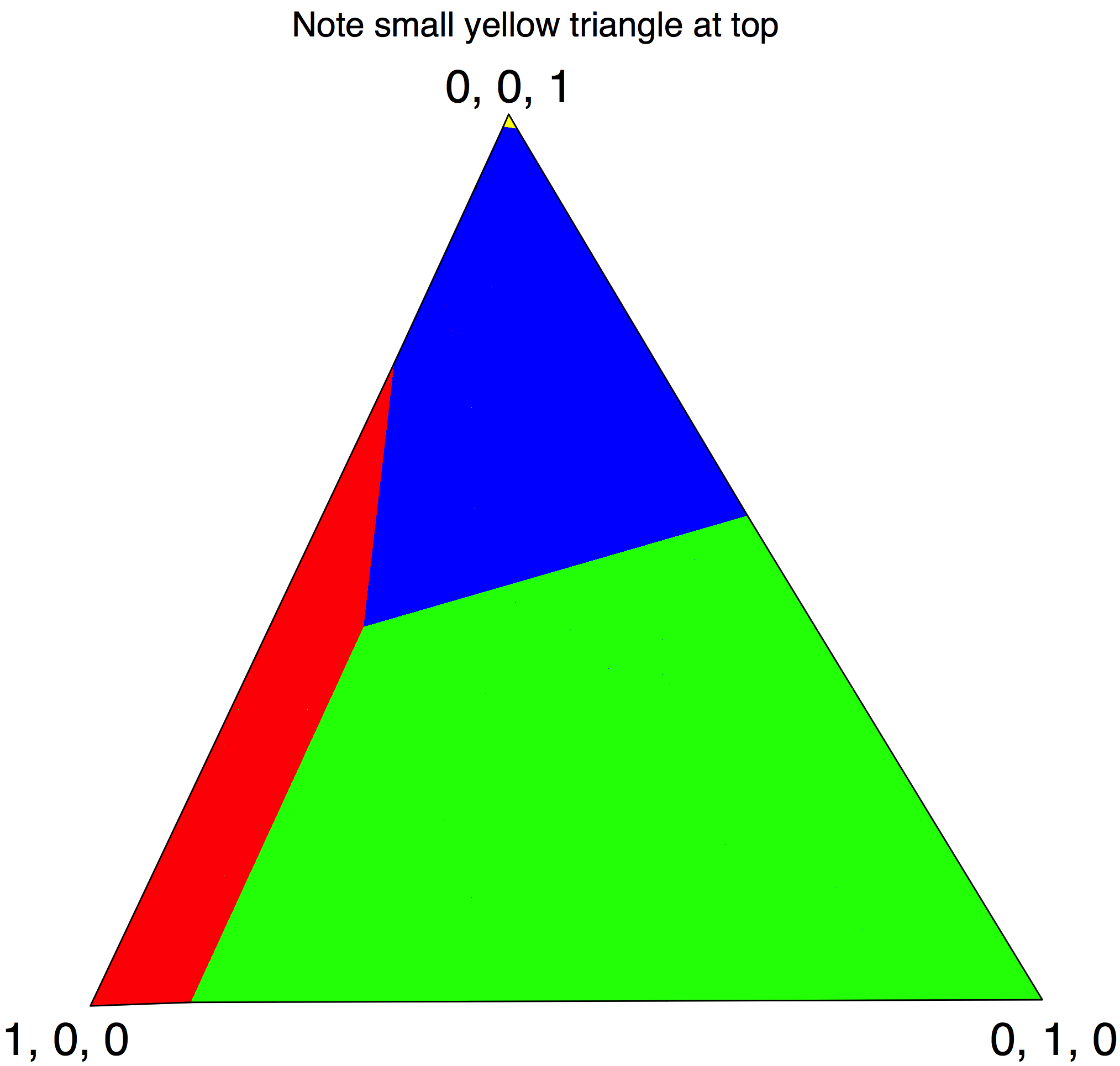
6.5) Belief-simplex policy regions§

The figure below partitions the belief simplex (vertices labeled shallow oil, deep oil, no oil) according to which fixed policy is best among four candidates. Match each region color to the policy.

5. In the yellow region, which policy is optimal among the four?

   	Always drill shallow
   	Always drill deep
   	Always give up
   	Test; if oil then deep else give up

   

6. In the blue region, which policy is optimal?

   	Always drill shallow
   	Always drill deep
   	Always give up
   	Test; if oil then deep else give up

   

7. In the red region, which policy is optimal?

   	Always drill shallow
   	Always drill deep
   	Always give up
   	Test; if oil then deep else give up

   

8. In the green region, which policy is optimal?

   	Always drill shallow
   	Always drill deep
   	Always give up
   	Test; if oil then deep else give up

   

7) Real world applications§

Partially Observable Markov Decision Processes (POMDPs) and multi-armed bandits are widely used for sequential decision-making under uncertainty. In healthcare, POMDPs can model patient treatment planning where the true health state is not fully observable, guiding clinicians to choose optimal interventions based on noisy test results. Multi-armed bandits appear in recommendation systems, such as in online advertising or streaming platforms, to balance exploration of new content and exploitation of known preferences. In robotics, POMDPs help autonomous systems stay robust despite sensor noise or occlusions.

8) Feedback§

1. How many hours did you spend on this homework?

   -- 2 3 4 5 6 7 8 more

   

2. Do you have any comments or suggestions (about the problems or the class)?