HW 5 -- MCTS and PDDL
Please Log In for full access to the web site.
Note that this link will take you to an external site (https://shimmer.mit.edu) to authenticate, and then you will be redirected back to this page.
This week's Colab notebook can be found here: Colab Notebook (Click Open with Google Colaboratory!)
1) Moving in Fractals §
We now introduce you to a family of reward problems --- we will call these fractal problems. Make sure you familiarize yourself with these problems since some of the following questions depend on them!
Fractal Problem A fractal problem is a reward problem with a finite horizon H such that:
- The state space \mathcal{S} is the entire plane \mathbb{R}^2
- The action at each time step t (assuming the agent takes the first action at step t=1) moves to one of the eight neighboring directions, with length scaled down by 2^{-t}:
\left\{(dx, dy) \mid (dx, dy) \in \{-2^{-t}, 0, 2^{-t}\}^2 \land (dx, dy) \neq (0, 0) \right\}
- The initial state is the origin at (0, 0).
- The entire state space is covered by a reward field. A reward field is a function that maps each point in the state space to a scalar reward: \mathbb{R}^2 \rightarrow \mathbb{R}^+.
In this problem, we will consider fractal problems with horizon H = 6 (that is, the agent is allowed to step 6 times).
1.1) Visualize Reward Fields§
We have defined for you three fractal problems in get_fractal_problems().
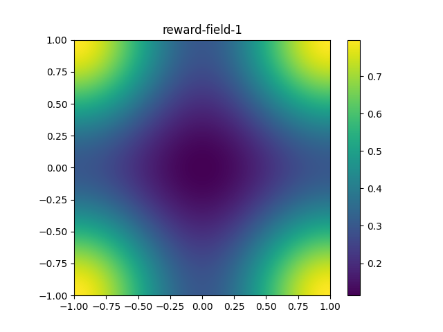
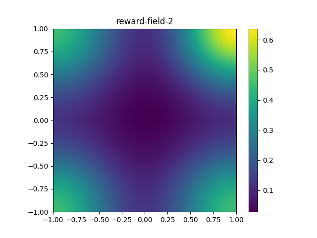
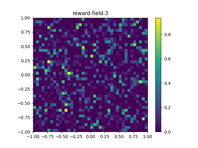
Below you can visualize the reward fields corresponding to these problems.
We have also provided you with code in the Colab notebook to recreate these visualizations.
You are encouraged to inspect the relevant class definitions for these problems to understand them better.
You do not need to submit any code for this subsection.
Instead, we will ask you questions in the following problems to confirm your understanding.
Once you are ready, let's confirm that you understand these reward fields:
-
What does
reward-field-1look most similar to?A smoothly changing gradient, where the four corners are equal local maxima. A smoothly changing gradient, where the four corners are equal local minima. A smoothly changing gradient, where the four corners are local maxima. Further, one corner's value is greater than the other three corners' values. A smoothly changing gradient, where the four corners are local minima. Further, one corner's value is less than the other three corners' values. Some noise. -
What does
reward-field-2look most similar to?A smoothly changing gradient, where the four corners are equal local maxima. A smoothly changing gradient, where the four corners are equal local minima. A smoothly changing gradient, where the four corners are local maxima. Further, one corner's value is greater than the other three corners' values. A smoothly changing gradient, where the four corners are local minima. Further, one corner's value is less than the other three corners' values. Some noise. -
What does
reward-field-3look most similar to?A smoothly changing gradient, where the four corners are equal local maxima. A smoothly changing gradient, where the four corners are equal local minima. A smoothly changing gradient, where the four corners are local maxima. Further, one corner's value is greater than the other three corners' values. A smoothly changing gradient, where the four corners are local minima. Further, one corner's value is less than the other three corners' values. Some noise. -
What is your best guess for the optimal plan for the problem
reward-field-2? You may take any guess --- we will grade any nonempty answer as correct. But we will ask you again later!Move towards the upper-right corner. Move towards the lower-left corner. Move towards any corner. Move towards the origin after taking a random initial step.

1.2) Path-cost Problem from Reward Problem§
Implement the reduction from a reward problem to a path-cost problem as in lecture.
For reference, our solution is 31 line(s) of code.
You should now be able to solve reward problems by using the above reduction and the uniform cost search implementation from the previous section.
reward-field-2? You should use path_cost_problem_from_reward_problem, run_uniform_cost_search and visualize_plan to help answer this question.| Move towards the upper-right corner. | |
| Move towards the lower-left corner. | |
| Move towards any corner. | |
| Move towards the origin after taking a random initial step. |
2) Play with MCTS§
2.1) Monte-carlo Warmup §
Consider the problem of finding the maximum value in an array of size n without duplicates.
-
The expected complexity of solving this problem by systematic search (i.e., by enumerating the array) is O(\underline{\quad\quad}).
Fill in the blank above. (Enter an expression in n. Hint: don't overthink --- it's not a trick question). -
Consider solving this problem by sampling uniformly at random with replacement.
import random, math
def find_max_random(array):
    best, seen = -math.inf, set()
    while len(seen) < len(array):
        x = random.choice(array)
        if x > best:
            best = x
        seen.add(x)
    return best
Let's think about the expected number of samples required for find_max_random to find the maximum value.
If we knew in advance what the maximum value was, then we would just draw samples at random until we hit the value we were looking for. The expected number of samples required to hit a particular element of a set of size n is just the expected number of trials required to get heads, when flipping a coin with probability 1/n of coming up heads. According to facts about the geometric distribution, the expected number of trials required before winning is 1 / (1/n) = n.
But we don't know what the maximum value is, so we can't stop as soon as we have encountered it! So, let's walk through another approach to the problem.
Along the way, we will leave some blanks for you to fill in.
Derivation
To be sure of finding the maximum value, find_max_random has to visit all n elements by uniformly sampling.
Let t_i be the time at which the algorithm first visits the i-th new index in the array (using 1-based indexing). In other words, t_i is the number of iterations of the while loop after len(seen) is incremented to i.
So, for example, if the sequence of (randomly) visited indices is [4, 2, 4, 4, 5, 2, 5, 6, \dots], then t_1 = 1 and [t_2, t_3, t_4] = \underline{ \quad \mathsf{A} \quad }.
\mathsf{ A }.
Let d_i be the number of samples the algorithm takes to find the i-th new index after it has found the i-1-th new index.
That is d_i = t_i - t_{i-1} for i > 1, and d_1 = 1. So, for example, in the list of visited indices above, d_1 = 1 and [d_2, d_3, d_4] = \underline{ \quad \mathsf{B} \quad }.
\mathsf{ B }.
\mathsf{ C }.
| d_1 + d_2 + \dots + d_{n-1} | |
| d_1 + d_2 + \dots + d_n | |
| d_1 + d_2 + \dots + d_{n+1} |
\mathsf{ D }.
| The expectation of a sum of random variables is the sum of the expectations of the individual random variables | |
| The expectation of a product of random variables is the product of the expectations of the random variables | |
| The expectation of any function of random variables is that function of the expectations of the random variables |
Let’s think about \mathbb{E}[d_i] now!
Suppose the algorithm has already found i-1 of the values and there are n total possible values.
So the probability that the algorithm would draw a new value by sampling uniformly at random for one step is \underline{ \quad \mathsf{E} \quad }.
\mathsf{ E }.
\mathsf{ F }.
\mathsf{ G }.
- when n = 10, \mathbb{E}[t_{10}] = \underline{ \quad \mathsf{H} \quad }.
\mathsf{ H }.
Fill in the blank \mathsf{ H } above. (Enter a number accurate to 2 decimal places)
- when n = 100, \mathbb{E}[t_{100}] = \underline{ \quad \mathsf{I} \quad }.
\mathsf{ I }.
Fill in the blank \mathsf{ I } above. (Enter a number accurate to 2 decimal places)
Conclusion. Under what circumstances does random sampling dominate systematic search in a problem like this? Answer: never! This problem is actually known as Coupon Collector's problem and the expected number of trials grows as \Theta(n log(n)) where n is the number of "coupons."
2.2) Practice with the upper confidence bound (UCB) §
Consider MCTS on a problem where the initial state s_0 has two actions a_0 and a_1. The UCB parameter C is 1.4. Suppose the search has completed 8 full iterations:
- It selected action a_0 3 times, receiving utilities [0.1, 0.7, 0.3].
- It selected action a_1 5 times, receiving utilities [0.4, 0.4, 0.4, 0.4, 0.4].
-
On the 9-th iteration, what is the UCB value for action a_0 when expanding from s_0? (Enter a number accurate to 2 decimal places)
-
On the 9-th iteration, what is the UCB value for action a_1 when expanding from s_0? (Enter a number accurate to 2 decimal places)
-
Which of the two actions will be selected on the 9-th iteration?
a_0 a_1
2.3) MCTS vs. UCS§
We have provided you an implementation of MCTS for reward problems in the Colab notebook. You should make sure that you can run our implementation on the reward problems we have defined for you. You are also encouraged to look into our code to see under how our MCTS is implemented. You do not need to submit any code for this question. Instead, we will ask you some questions to confirm your understanding.
2.3.1) Which will work better?§
For each of the problems defined in get_fractal_problems, what is your best guess of if MCTS or UCS (uniform cost search) will work better?
For concreteness, by "work better" we mean the expected number of problem.step invocations to find an optimal plan.
-
What is your guess of which one will work better for
reward-field-1? You may take any guess --- we will grade any nonempty answer as correct.MCTS UCS -
What is your guess of which one will work better for
reward-field-2? You may take any guess --- we will grade any nonempty answer as correct.MCTS UCS -
What is your guess of which one will work better for
reward-field-3? You may take any guess --- we will grade any nonempty answer as correct.MCTS UCS
2.3.2) Compare the performance§
Now, for each of the problems defined in get_fractal_problems, let us compare the performances of MCTS vs. UCS empirically by running run_mcts_search and run_uniform_cost_search.
In particular, you should:
- Fix
step_budgetfor both algorithms to 2500. Setiteration_budgetfor MCTS to infinity. - Run MCTS 20 times and record the average cumulative reward.
- Run UCS once:
- If it fails (due to running out of step budget), record the cumulative reward as 0.
- If it succeeds, record the obtained cumulative reward. Hint: you might need to recover rewards from path costs
- Repeat the above for all three problems in
get_fractal_problems.
-
What is the average cumulative reward obtained by MCTS in
reward-field-1? -
What is the obtained cumulative rewards by UCS in
reward-field-1? -
What is the average cumulative reward obtained by MCTS in
reward-field-2? -
What is the obtained cumulative rewards by UCS in
reward-field-2? -
What is the average cumulative reward obtained by MCTS in
reward-field-3? -
What is the obtained cumulative rewards by UCS in
reward-field-3? -
MCTS tends to be a better choice than UCS when: (choose all that apply)
There is a single high-valued state and everything else has value 0. The value of the first part of a path gives you information about the value of its completions. You would rather have an "okay" answer soon than the optimal answer after a longer period of time.
2.4) Adjusting C in MCTS §
2.4.1) Choosing C§
Consider the following scenarios:
- An early trajectory has a terrible outcome and the algorithm never tries its initial action again.
- The algorithm behaves very similarly to a systematic enumeration of all possible paths.
- The algorithm behaves very similarly to a systematic enumeration of all possible path prefixes, with each followed by a random completion.
For each of the scenarios, indicate whether:
- It is likely to happen when C is too high.
- It is likely to happen when C is too low.
- It is unlikely to happen in MCTS.
-
An early trajectory has a terrible outcome and we never try its initial action again.
It is likely to happen when C is too high. It is likely to happen when C is too low. It is unlikely to happen in MCTS. -
The algorithm behaves very similarly to a systematic enumeration of all possible paths.
It is likely to happen when C is too high. It is likely to happen when C is too low. It is unlikely to happen in MCTS. -
The algorithm behaves very similarly to a enumeration of all possible path prefixes, with each followed by a random completion.
It is likely to happen when C is too high. It is likely to happen when C is too low. It is unlikely to happen in MCTS.
3) Warming up with Pyperplan§
In this homework, we will be using a Python PDDL planner called pyperplan.
Let's warm up by using pyperplan to solve a given blocks PDDL problem.
3.1) Let's Make a Plan§
Use run_planning to find a plan for the blocks problem defined at the top of the colab file (BLOCKS_DOMAIN, BLOCKS_PROBLEM).
The run_planning function takes in a PDDL domain string, a PDDL problem string, the name of a search algorithm, and the name of a heuristic (if the search algorithm is informed) or a customized heuristic class. It then uses the Python planning library pyperplan to find a plan.
The plan returned by run_planning is a list of pyperplan Operators. You should not need to manipulate these data structures directly in this homework, but if you are curious about the definition, see here.
The search algs available in pyperplan are: astar, wastar, gbf, bfs, ehs, ids, sat. The heuristics available in pyperplan are: blind, hadd, hmax, hsa, hff, lmcut, landmark.
For this question, use the astar search algorithm with the hadd heuristic.
For reference, our solution is 2 line(s) of code.
3.2) Fill in the Blanks§
You've received PDDL domain and problem strings from your boss and you need to make a plan, pronto! Unfortunately, some of the PDDL is missing.
Here's what you know. What you're trying to model is a newspaper delivery robot. The robot starts out at a "home base" where there are papers that it can pick up. The robot can hold arbitrarily many papers at once. It can then move around to different locations and deliver papers.
Not all locations want a paper -- the goal is to satisfy all the locations that do want a paper.
You also know:
- There are 6 locations in addition to 1 for the homebase. Locations 1, 2, 3, and 4 want paper; locations 5 and 6 do not.
- There are 8 papers at the homebase.
- The robot is initially at the homebase with no papers packed.
Use this description to complete the PDDL domain and problem. You can assume the PDDL planner will find the optimal solution.
If you are running into issues writing or debugging the PDDL you can check out this online PDDL editor, which comes with a built-in planner: editor.planning.domains. To use the editor, you can create two files, one for the domain and one for the problem. You can then click "Solve" at the top to use the built-in planner.
For a general reference on PDDL, check out planning.wiki. Note that the PDDL features supported by pyperplan are very limited: types and constants are supported, but that's about it. If you want to make a domain that involves more advanced features, you can try the built-in planner at editor.planning.domains, or you can use any other PDDL planner of your choosing.
Debugging PDDL can be painful. The online editor at editor.planning.domains is helpful: pay attention to the syntax highlighting and to the line numbers in error messages that result from trying to Solve. To debug, you can also comment out multiple lines of your files by highlighting and using command+/. Common issues to watch out for include:
- A predicate is not defined in the domain file
- A variable name does not start with a question mark
- An illegal character is used (we recommended sticking with alphanumeric characters, dashes, or underscores; and don't start any names with numbers)
- An operator is missing a parameter (in general, the parameters should be exactly the variables that are used anywhere in the operator's preconditions or effects)
- An operator is missing a necessary precondition or effect
- Using negated preconditions, which are not allowed in basic Strips
If you get stuck debugging your PDDL file for more than 10-15 min, please reach out and we'll help!
For reference, our solution is 89 line(s) of code.
4) Planning Heuristics§
Let's now compare different search algorithms and heuristics.
Let's consider two of the search algorithms available in pyperplan:
astar, gbf. (gbf stands for greedy-best-first search.)
And the following heuristics: blind, hadd, hmax, hff, lmcut. blind, hmax and lmcut are admissible; hadd and hff are not.
Unfortunately the documentation for pyperplan is limited at the moment, but if you are curious to learn more about its internals, the code is open-sourced on this GitHub repo.
4.1) Comparison§
We have given you a set of blocks planning problem of different complexity BW_BLOCKS_PROBLEM_1 to BW_BLOCKS_PROBLEM_6.
You can use the function test_run_planning found in the Colab to test the different combinations of search and heuristic
on different problems. There is also a helper function in the Colab to plot the result.
If planning takes more than 30 seconds, just kill the process.
| Problems 1, 2 and 3 are easy (plan in less than 30 seconds) for all the methods. | |
| Problem 4 is easy (plan in less than 30 seconds) for all the non-blind heuristics. | |
Problem 4 is easy (plan in less than 30 seconds) for all the non-blind heuristics, except hmax. | |
The blind heuristic is generally hopeless for the bigger problems. | |
hadd is generally much better (leads to faster planning) than hmax. | |
gbf-lmcut will always find paths of the same length as astar-lmcut (given sufficient time). | |
astar-lmcut will always find paths of the same length as astar-hmax (given sufficient time). | |
astar-lmcut usually finds paths of the same length as astar-hff (in these problems). | |
gbf-hff is a good compromise for planning speed and plan length (in these problems). |
4.2) Relax, It's Just Logistics§
Consider the PDDL domain for logistics.
We create a delete-relaxed version of the logistics domain by dropping the negative effects from each operator.
Now we want to compute h^{\textit{ff}} for this initial state and goal
    I = {truck(t), package(p), location(a), location(b),
         location(c), location(d), location(e),
         at(t, a), at(p, c),
         road(a, b), road(b, c), road(c, d), road(a, e),
         road(b, a), road(c, b), road(d, c), road(e, a)}

    G = {at(t, a), at(p, d)}.
-
What are the actions in the relaxed plan that we would extract from the RPG for this problem, using the h^{\textit{ff}} algorithm? Enter the plan as a list of strings; ordering is not important.
Enter a list of strings, e.g.["drive-truck(t,a,b)", "unload-truck(p,t,d)"].
-
What is the value of the heuristic score of the initial state: h^{\textit{ff}}(I)?
Enter an integer
4.3) More Relaxing Fun§
| If there exists a plan to achieve a goal with a single fact \{\texttt{g}\}, then that fact \texttt{g} must appear in some level of the relaxed planning graph (RPG). | |
| If there exists a plan to achieve a goal with a single fact \{\texttt{g}\}, then that fact \texttt{g} must appear in the last level of the RPG. | |
| The last level of the RPG is a superset of all of the facts that could ever be in the state by taking actions from the initial state. | |
| The initialization (initial state) of the RPG may affect the number of levels in the RPG, but it will not change the final set of facts in the last level of the RPG. | |
| If a fact \texttt{g} appears in some level of the RPG, then there exists a (non-relaxed) plan to achieve the goal \{\texttt{g}\}. |
5) Implementing h^{\textit{ff}}§
In the code below, one of the arguments is a Pyperplan Task instance.
Please study these definitions; some of the methods may be useful in writing your code. Note that fact names are strings as are the names of Operator instances.
Also, note that most of the attributes are frozenset; if you want to modify them, you can do set(x) to convert a frozenset x to a set.
5.1) Construct Reduced Planning Graph (RPG)§
Given a Pyperplan Task instance and an optional state, return (F_t, A_t), two lists as defined in the RPG pseudo-code from lecture. Note that fact names in the documentation of Task are strings such as '(on a b)' and operator instances are instances of the Operator class; the name of an operator instance is a string such as '(unstack a c)'. If state is None, use task.initial_state.
For reference, our solution is 15 line(s) of code.
5.2) Implement h_add§
Given a Pyperplan Task instance and a state (set of facts or None), return h_add(state).
For reference, our solution is 7 line(s) of code.
In addition to all the utilities defined at the top of the Colab notebook, the following functions are available in this question environment: construct_rpg. You may not need to use all of them.
5.3) Implement h_ff (OPTIONAL)§
Given a Pyperplan Task and a state (set of facts or None), return h_ff(state).
For reference, our solution is 26 line(s) of code.
In addition to all the utilities defined at the top of the Colab notebook, the following functions are available in this question environment: construct_rpg. You may not need to use all of them.
6) Feedback§
-
How many hours did you spend on this homework?
-
Do you have any comments or suggestions (about the problems or the class)?