HW 3 -- Kalman Filters & Approximate Inference
Please Log In for full access to the web site.
Note that this link will take you to an external site (https://shimmer.mit.edu) to authenticate, and then you will be redirected back to this page.
This week's Colab notebook can be found here: Colab Notebook (Click Me!)
1) Gaussians§
1.1) §
| A + B | |
| 10A - 12B | |
| A \times B | |
| The joint distribution of A and B |

Let A \sim \mathcal{N}(\mu_A, \sigma_{A}^{2}) and let B | A \sim \mathcal{N} (A, \sigma^{2}_{B|A}). We can show the distribution A | B = b is a univariate Gaussian.
For parsing purposes, enter \mu_A as mu_A, \sigma_{A} as sigma_A, \sigma_{B \mid A} as sigma_BA, b as b, and the ^ character for exponentation.
1.2) §
1.3) §
1.4) §
| True | |
| False |
1.5) §
| True | |
| False |
2) Continuous PGMs §
Consider a Bayesian network with three one-dimensional continuous variables: A, B, and C. Let A \sim \mathcal{N}(1, 1), B \sim \mathcal{N}(2, 4), and C \sim \mathcal{N}(A + B, 1).
2.1) §
2.2) §
2.3) §
2.4) §
Hint: We can apply linearity of covariance to compute Cov(A,C) and Cov(B, C).
2.5) §
2.6) §
2.7) §
Hint: See Lec06 slide 12 for the general formula of the covariance matrix for Bayesian networks.
2.8) §
2.9) §
| Independent | |
| Not independent |
2.10) §
| Conditionally independent | |
| Not conditionally independent |
3) HMMs: Are my leftovers (still) edible? §
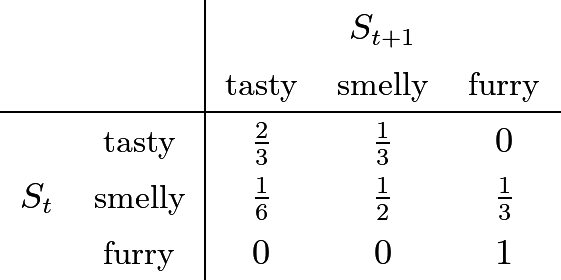
I use an HMM to model the state of my leftover food over time. The state space is \{\textit{tasty}, \textit{smelly}, \textit{furry} \}. Initially, I'm sure they're tasty: P(S_0 = \textit{tasty}) = 1. The state transition model is:
3.1) Sampling Formulas §
You decide to estimate P(S_2) by forward (prior) sampling. You generate 100 sample trajectories of length 3 for your leftovers. Given those trajectories what are the three terms to construct an estimate of P(S_2)?
| (number of trajectories ending in tasty)/100 | |
| (number of trajectories with tasty)/100 | |
| (number of trajectories ending in smelly)/100 | |
| (number of trajectories with smelly)/100 | |
| (number of trajectories ending in furry)/100 | |
| (number of trajectories with furry)/100 |
| (number of trajectories ending in tasty)/100 | |
| (number of trajectories with tasty)/100 | |
| (number of trajectories ending in smelly)/100 | |
| (number of trajectories with smelly)/100 | |
| (number of trajectories ending in furry)/100 | |
| (number of trajectories with furry)/100 |
| (number of trajectories ending in tasty)/100 | |
| (number of trajectories with tasty)/100 | |
| (number of trajectories ending in smelly)/100 | |
| (number of trajectories with smelly)/100 | |
| (number of trajectories ending in furry)/100 | |
| (number of trajectories with furry)/100 |
4) Properties of Viterbi§
Maximillian thinks the Viterbi algorithm is too complicated and we could get away without the backward “decoding” pass, and instead just return the maximum of the marginal distribution at each time step.
You know better than Max! In the HMM below, provide a sequence of three observations for which Max will get the wrong answer, but Viterbi decoding will be correct Your answer should be a Python list of three True/False values. Assume that the initial distribution is uniform.
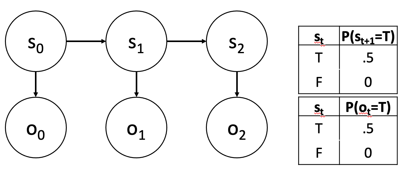
[True, True, True].
5) HMMs and Kalman Filters§
| The forward-backward algorithm for HMMs is exactly the same algorithm as the Viterbi algorithm. | |
| The forward-backward algorithm for HMMs is a special case of the sum-product algorithm. | |
| The Viterbi algorithm for HMMs is a special case of the max-product algorithm. | |
| Forward-backward is linear in the number of time steps. | |
| Filtering to maintain a state estimate after each new observation requires us to store the history of all forward messages. | |
| Running smoothing in an HMM efficiently to update estimates of past states after each new observation requires us to store the history of all forward messages. | |
| Kalman filtering requires, for each time step, a number of multiplication operations that is roughly cubic in the number of state variables. | |
| HMM filtering requires, for each time step, a number of multiplication operations that is roughly cubic in the size of the domain of the observation variable. | |
| Kalman filtering can be used to determine the true most likely state estimate at time t when the state is continuous and the transition and observation dynamics are linear and Gaussian. | |
| In Kalman filtering, if we only care about the maximum likelihood state estimate at time t, and not the covariance of our estimate, we don't need to compute the covariances at previous time steps. | |
| We can use an HMM model and algorithm to find an exact solution for the most likely state estimate at time t when the state is continuous and the transition and observation dynamics are linear and Gaussian. | |
| If we are using a HMM to make decisions at each timestep t, we only need to store the marginal over the state s_{t-1}, the transition potential from s_{t-1} to s_t and the measurement potential from o_t to s_t. |
6) Kalman Filtering§
Consider the following one-dimensional continuous-state system:
where w_t \sim N(0, \sigma_w^2) and v_t \sim N(0, \sigma^2_v). This is the same linear-Gaussian model that we discussed in lecture, but we now have a control input u_t.
Let us say that a = 2, h = 10, \sigma^2_w = 1 and \sigma^2_v = .25. Let us also say that the initial estimate of the state is
-
Given a single action u_0 = 1, what is the mean of x_1?
Enter a number that is accurate to within 1.0e-5. You can also enter a python expression that will evaluate to a number (e.g.,3*2 + 4 - 7/11.0). -
Given a single action u_0 = 1, what is the variance of x_1?
Enter a number that is accurate to within 1.0e-5. You can also enter a python expression that will evaluate to a number (e.g.,3*2 + 4 - 7/11.0). -
After the action u_0 = 1, what is the expected measurement y_1?
Enter a number that is accurate to within 1.0e-5. You can also enter a python expression that will evaluate to a number (e.g.,3*2 + 4 - 7/11.0). -
Given a subsequent measurement y_1 = 0, what is the variance of the posterior on x_1?
Enter a number that is accurate to within 1.0e-5. You can also enter a python expression that will evaluate to a number (e.g.,3*2 + 4 - 7/11.0). -
Given a subsequent measurement y_1 = 0, what is the mean of the posterior on x_1?
Enter a number that is accurate to within 1.0e-5. You can also enter a python expression that will evaluate to a number (e.g.,3*2 + 4 - 7/11.0). -
The covariance of the posterior will ...
always get smaller over time always get bigger over time get bigger or smaller over time depending on the relative magnitudes of a to h get bigger or smaller over time depending on the relative magnitudes of \sigma_w to \sigma_v
7) Coding: Kalman Filter§
Let's implement the Kalman Filter for the one-dimensional continuous-state system from the previous section.
7.1) Kalman Filter Warmup§
Return an Gaussian object with mean=0, std=2.
Please see the provided code for the definition of Gaussian.
For reference, our solution is 1 line(s) of code.
7.2) Kalman filter process model§
Implement the process step of a 1D Kalman filter, given a Gaussian prior distribution, a process model a, \sigma^2_w, and a control u.
For reference, our solution is 4 line(s) of code.
7.3) Kalman filter measurement model§
Implement the measurement step of a 1D Kalman filter, given a prior mean and variance, a measurement model h, \sigma^2_v, and a received measurement y.
For reference, our solution is 18 line(s) of code.
7.4) Kalman filter§
Combine the process and measurement steps into a single estimator that takes a prior, a process model, a measurement model, a list of controls, measurements, and returns a posterior.
For reference, our solution is 9 line(s) of code.
In addition to all the utilities defined at the top of the Colab notebook, the following functions are available in this question environment: kf_measurement, kf_process. You may not need to use all of them.
7.5) Kalman Filter Visualization§
We have created a visualization tool in Colab for the filtering process. You can run the code blocks and an animation of the filtered Gaussian in each step will be shown. There is also a plot showing the line chart of ground-truth locations, measurements, and posteriors.
Run the animation that visualizes the distribution of x_t after each process update and observation update. Use the "next frame" button (to the right of "play") to see what happens one step at a time.
Now look at the plot below the animation. The plot shows a green region that is the Kalman filter's mean +/- one stdev for each timestep after the observation update.
| As time passes, the green area will shrink. | |
| As time passes, the measurements (in orange) will stay inside the green region. | |
| As time passes, the Kalman filter mean will get closer to the ground truth. |
8) Sampling§
8.1) Sampling types§
| In the limit of infinite samples, the statistics we compute from a set of samples generated by Gibbs sampling, such as the mean of a variable, match the statistics of the underlying distribution. | |
| It is possible to know ahead of time how many samples will be needed for importance sampling. | |
| For some samplers, it is possible to know at execution time, by measuring the total weight of the samples collected so far, whether more samples are needed | |
| When computing importance weights w(X) = P(X)/Q(X) for a sample X, it is important that P(X) be correctly normalized. | |
| It is important that the potentials in the graphical model are correctly normalized for sampling to work. | |
| We need to know ahead of time the statistics of the target distribution when designing the proposal distribution for importance sampling. | |
| A bad proposal distribution means more samples from the proposal distribution will be needed to get a good estimate of the target distribution. | |
| We don't need to worry about the direction of arrows when Gibbs sampling in a Bayes net. | |
| The samples generated by Gibbs sampling are independent and identically distributed. |
8.2) Sampling efficiency§
Kullback-Leibler divergence is an estimate of how similar two distributions are, and for discrete distributions it is given by
Let us assume that P is the target distribution, and Q is the proposal distribution, and we are performing rejection sampling.
What does this mean for our sampling strategy?
| When Q(x) is small for x\in {\mathcal {X}} where P(x) is large, D_{KL}(P||Q) will always be large. | |
| When Q(x) is large for x\in {\mathcal {X}} where P(x) is small, D_{KL}(P||Q) will always be large. | |
| When D_{KL}(P||Q) is large, the sampling strategy will be very good. P and Q are closely aligned. | |
| When D_{KL}(P||Q) is small, the sampling strategy will be very good no matter what. P and Q are closely aligned. | |
| Our sampling strategy will be efficient when the KL divergence is small and P(x) isn't small or zero for x where Q(x) is large. | |
| If Q has zero probability in places where P is non-zero, we will not get a representative set of samples. |
9) More Sampling§
9.1) Gibbs Sampling§
Consider the following 3 node factor graph: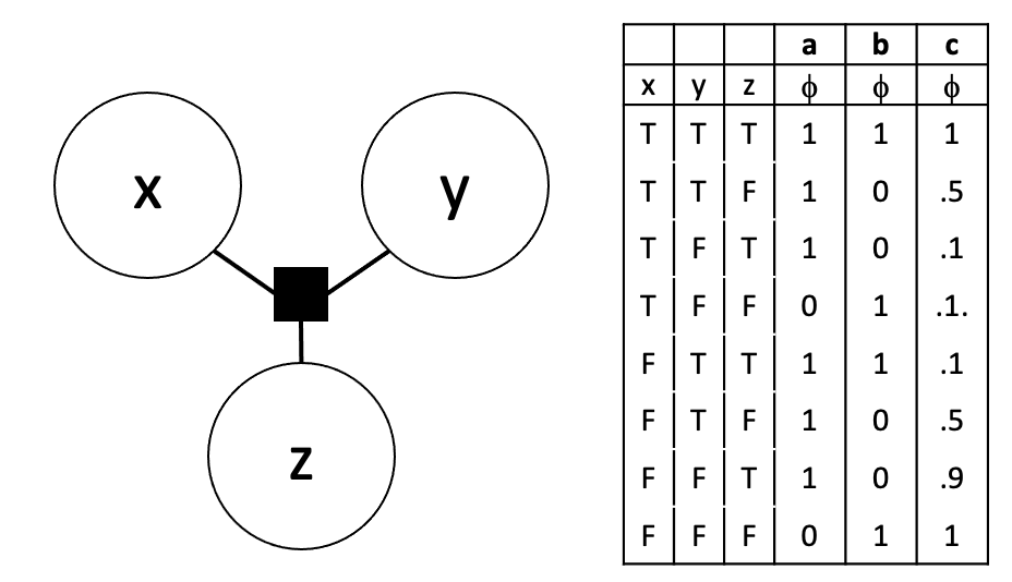
The table on the right gives three different potential tables for the factor. Gibbs sampling did a poor job on generating samples that reflected the joint of these three variables for one of these potential tables. Which was it?
| a | |
| b | |
| c |
9.2) Sampling in Bayes net§
Consider the following Bayes net.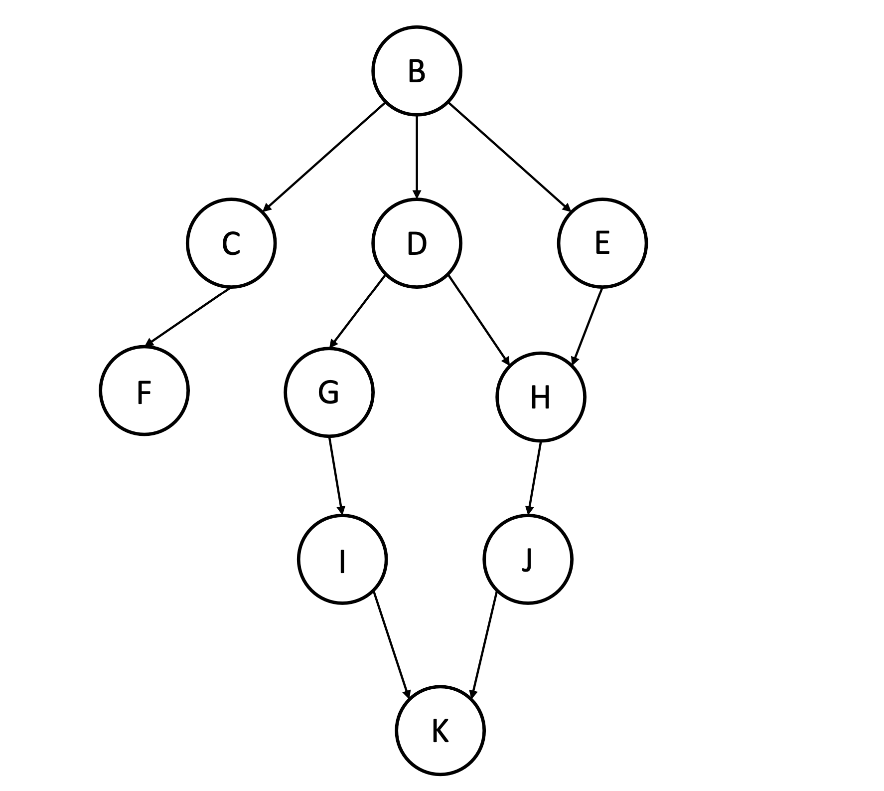
We are interested in drawing samples from the distribution described by this network, conditioned on evidence, using ancestral sampling with rejection.
-
Is this a good way to sample from P(K \mid B = b)?
True False -
Is this a good way to sample from P(B \mid K = k)?
True False
9.3) Markov Blanket§
Consider the Bayes net from the above question.
-
Enter the set of nodes in the Markov Blanket of node G, e.g.
['B','D']. -
Enter the set of nodes in the Markov Blanket of node D, e.g.
['B','D'].
10) Gibbs Sampling§
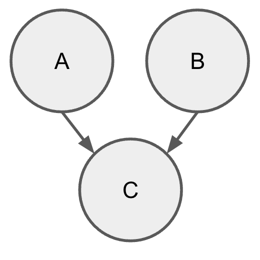
We are going to study Gibbs sampling in a concrete case, to illustrate some of the principles. Assume that we choose variables to change uniformly in the Gibbs procedure. Consider the following Bayes net with three binary variables, A, B, and C.
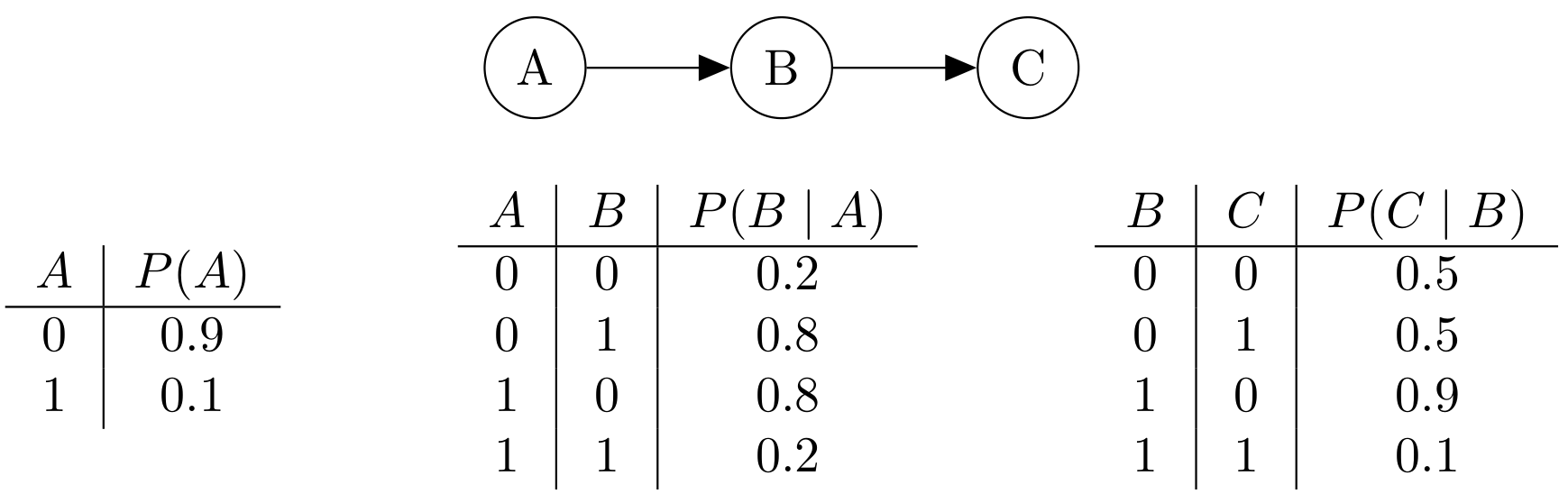
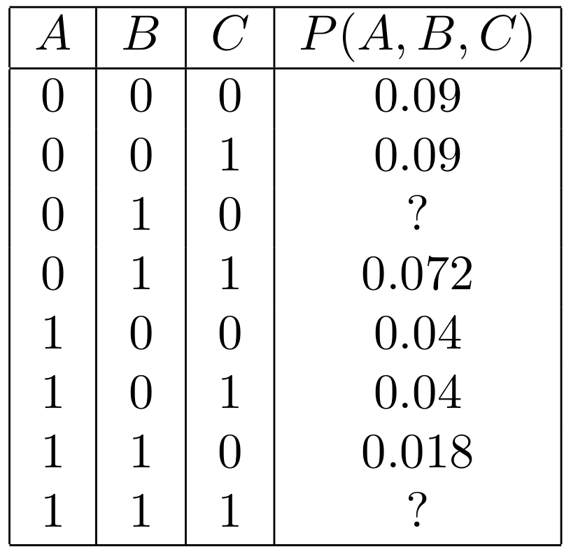
- What's the joint distribution? We've filled in most of the values for you.
- In Gibbs sampling, say we start with assignment (0, 0, 0). Let's calculate some probabilities of a single step.
- Now say we start with assignment (1, 0, 0).
- Recall that Gibbs sampling implicitly constructs a Markov chain where the states are assignments of values to variables, and T(x, x') is the probability of moving from x to x'. One step in showing that the true joint distribution of this model (\pi) is the stationary distribution of this Markov chain, is to show that, for all x and x', \pi(x) \cdot T(x, x') = \pi(x') \cdot T(x', x).This is called detailed balance, which implies stationarity because it says the probability leaving is the same as the probability entering on every iteration. Let's verify the equation holds for a pair of states.
11) Particle Filter§
Consider a domain in which the forward transition dynamics are “hybrid” in the sense that
that is, with probability p, the state will hop forward one unit in expectation, and with probability 1-p, it will hop backward one unit in expectation, with variance 0.1 in each case.
Assume additionally that the observation model P(Y_t = y_t \mid X_t = x_t) = \mathtt{Uniform}(x_{t}-1, x_{t}+1)(y_t)
-
What is E[X_t \mid X_{t-1} = x]?
x-2 x + 2p - 1 p^2 * x p * x -
Assuming p=0.5, what is Var[X_t \mid X_{t-1} = x]?
0.1 0.2 1.1 0.05 -
You know the initial state of the system X_0 = 0. Your friend Norm thinks it’s fine to initialize a particle filter with a single particle at 0. What do you think?
This is fine and we can continue with a single particle. We should initialize our pf with N copies of this particle. -
Norm runs the filter for two steps with no observations several times and is trying to decide whether there could be bugs in the code. Assuming p=0.5, for each of the following sets of particles, indicate whether it is (a) fairly likely (b) quite unlikely (c) completely impossible:
-
{-2.05, -1.95, -0.1, 0.1, 1.9, 2.1}
(a) fairly likely (b) quite unlikely (c) completely impossible -
{-2.01, -1.9, -1.0, 0.1, 0, 2.1}
(a) fairly likely (b) quite unlikely (c) completely impossible -
{-20, -2.01, -2.001, .01, .001, 1.99, 1.999}
(a) fairly likely (b) quite unlikely (c) completely impossible
-
-
Norm initializes the filter with particles {-2.05, -1.95, -0.1, 0.1, 1.9, 2.1} and then gets an observation of -1.0. Which of the following is a plausible posterior, assuming resampling without noise?
{-1.95, -0.1, -1.95, -1.95, -0.1, -0.1, -0.1} {-1.95, -.01} {0.1, 0.1, 0.1, -0.1, -0.1, -0.1} {-1.96, -0.11, -1.94, -1.97, -0.11, -0.09, -0.12}
11.1) Particle Filter Code and Visualization§
We've created a visualization and code simulation in Colab for this problem, using the same hybrid dynamics model at the start of this problem. You can run the code block to run the particle filter on the problem, experiment with different parameters, and plot the results.
| Particle exhaustion happens when the current observation is impossible given all the particles. | |
| Particle exhaustion happens when the current motion is impossible given all the particles. | |
| If we get data from the same actual system as described above, but changed the motion model in the particle filter to be a single Gaussian, then we would be less likely to experience particle exhaustion. | |
| If we get data from the same actual system as described above, but changed the observation model in the particle filter to be Gaussian (rather than uniform), we would be less likely to experience particle exhaustion. | |
| If we used fewer particles, we would be less likely to experience particle exhaustion. | |
| If we get data from the same actual system as described above, but changed the motion model in the particle filter to not have Gaussian noise (so moving +1 with probability p, and -1 with probability 1-p), then we would be more likely to experience particle exhaustion. |
Experiment with the number of particles. The animation shows the location of the particles and ground truth after each timestep. The line plot shows the location over time, as well as a green shaded region indicating the particle filter's mean +/- one stdev of the particles.
12) Feedback§
-
How many hours did you spend on this homework?
-
Do you have any comments or suggestions (about the problems or the class)?